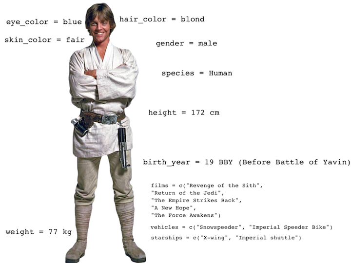
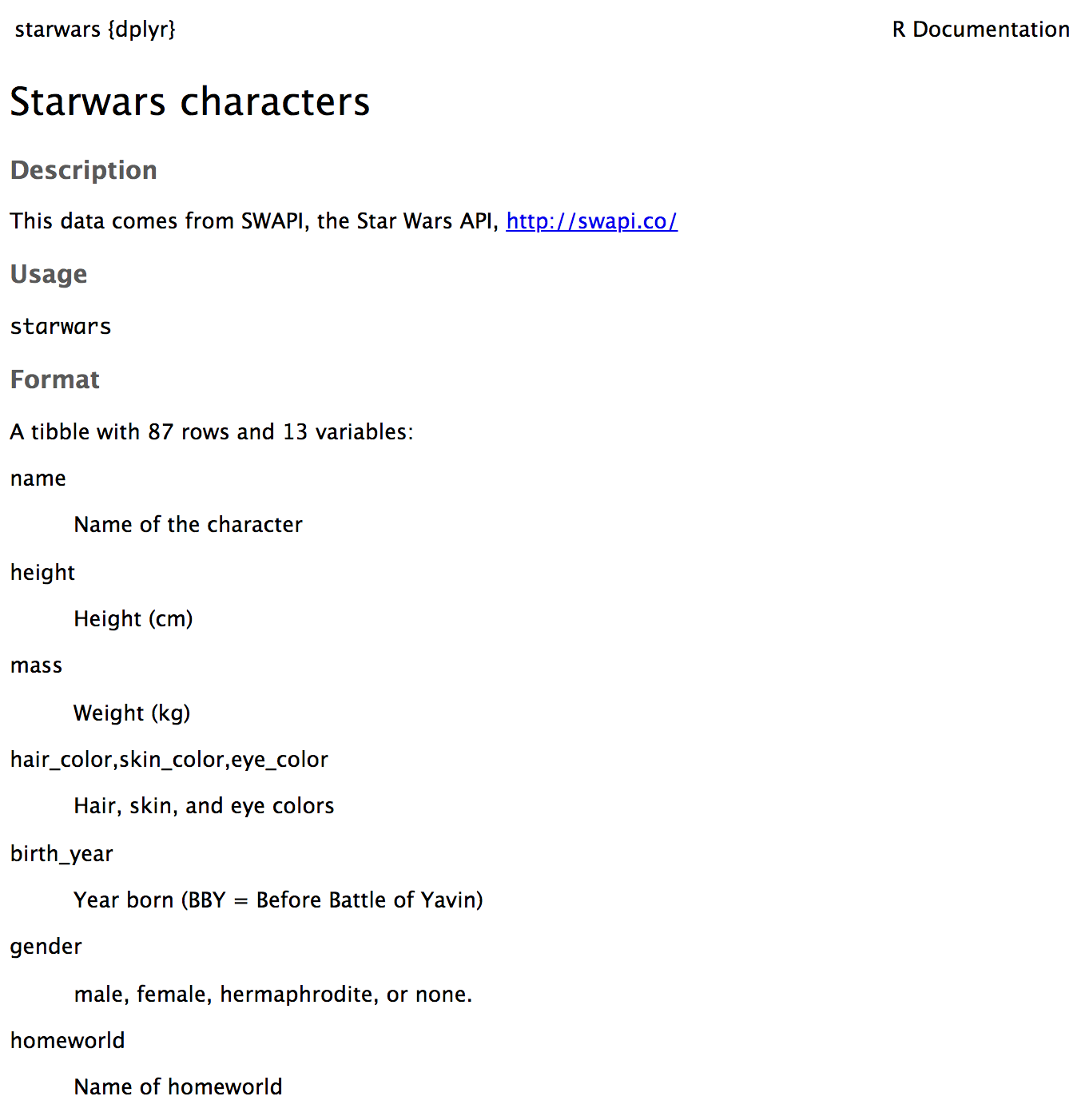
Exploratory Data Analysis and Why visualize ? 📊

# Exploratory Data Analysis and Why visualize ?<br> 📊

---

layout: true
  
<div class="my-footer">
<span>
<a href="" target="_blank">
</a>
</span>
</div>

---

# Exploratory data analysis

---

## What is EDA?

- Exploratory data analysis (EDA) is an aproach to analyzing data sets to summarize its main characteristics.
- Often, this is visual. That's what we're focusing on today.
- But we might also calculate summary statistics and perform data wrangling/manipulation/transformation at (or before) this stage of the 
analysis. That's what we'll focus on next.

---

# Star Wars Dataset

---

## Dataset terminology

- Each row is an **observation**
- Each column is a **variable**

```r
starwars
```

```
## # A tibble: 87 x 14
##    name  height  mass hair_color skin_color eye_color birth_year sex   gender
##    <chr>  <int> <dbl> <chr>      <chr>      <chr>          <dbl> <chr> <chr> 
##  1 Luke…    172    77 blond      fair       blue            19   male  mascu…
##  2 C-3PO    167    75 <NA>       gold       yellow         112   none  mascu…
##  3 R2-D2     96    32 <NA>       white, bl… red             33   none  mascu…
##  4 Dart…    202   136 none       white      yellow          41.9 male  mascu…
##  5 Leia…    150    49 brown      light      brown           19   fema… femin…
##  6 Owen…    178   120 brown, gr… light      blue            52   male  mascu…
##  7 Beru…    165    75 brown      light      blue            47   fema… femin…
##  8 R5-D4     97    32 <NA>       white, red red             NA   none  mascu…
##  9 Bigg…    183    84 black      light      brown           24   male  mascu…
## 10 Obi-…    182    77 auburn, w… fair       blue-gray       57   male  mascu…
## # … with 77 more rows, and 5 more variables: homeworld <chr>, species <chr>,
## #   films <list>, vehicles <list>, starships <list>
```
]

---

## Luke Skywalker

![luke-skywalker](img/luke-skywalker.png)

---

## What's in the Star Wars data?

Take a `glimpse` at the data:

```r
glimpse(starwars)
```

```
## Rows: 87
## Columns: 14
## $ name       <chr> "Luke Skywalker", "C-3PO", "R2-D2", "Darth Vader", "Leia O…
## $ height     <int> 172, 167, 96, 202, 150, 178, 165, 97, 183, 182, 188, 180, …
## $ mass       <dbl> 77.0, 75.0, 32.0, 136.0, 49.0, 120.0, 75.0, 32.0, 84.0, 77…
## $ hair_color <chr> "blond", NA, NA, "none", "brown", "brown, grey", "brown", …
## $ skin_color <chr> "fair", "gold", "white, blue", "white", "light", "light", …
## $ eye_color  <chr> "blue", "yellow", "red", "yellow", "brown", "blue", "blue"…
## $ birth_year <dbl> 19.0, 112.0, 33.0, 41.9, 19.0, 52.0, 47.0, NA, 24.0, 57.0,…
## $ sex        <chr> "male", "none", "none", "male", "female", "male", "female"…
## $ gender     <chr> "masculine", "masculine", "masculine", "masculine", "femin…
## $ homeworld  <chr> "Tatooine", "Tatooine", "Naboo", "Tatooine", "Alderaan", "…
## $ species    <chr> "Human", "Droid", "Droid", "Human", "Human", "Human", "Hum…
## $ films      <list> [<"The Empire Strikes Back", "Revenge of the Sith", "Retu…
## $ vehicles   <list> [<"Snowspeeder", "Imperial Speeder Bike">, <>, <>, <>, "I…
## $ starships  <list> [<"X-wing", "Imperial shuttle">, <>, <>, "TIE Advanced x1…
```

---

## What's in the Star Wars data?

.question[
How many rows and columns does this dataset have? What does each row represent? What does each column represent?
]

```r
?starwars
```

![](img/starwars-help.png)

---

#  EDA: 1. Identifying variables

---

## Number of variables involved

* Univariate data analysis - distribution of single variable
* Bivariate data analysis - relationship between two variables
* Multivariate data analysis - relationship between many variables at once, usually focusing on the relationship between two while conditioning for others

---

## Types of variables

- **Numerical variables** can be classified as **continuous** or **discrete** based on whether or not the variable can take on an infinite number of values or only non-negative whole numbers, respectively. 
- If the variable is **categorical**, we can determine if it is **ordinal** based on whether or not the levels have a natural ordering.

---

# Visualizing numerical data

---

## Describing shapes of numerical distributions

* shape:
    * skewness: right-skewed, left-skewed, symmetric (skew is to the side of the longer tail)
    * modality: unimodal, bimodal, multimodal, uniform
* center: mean (`mean`), median (`median`), mode (not always useful)
* spread: range (`range`), standard deviation (`sd`), inter-quartile range (`IQR`)
* unusal observations

---

## Histograms

```r
ggplot(data = starwars, mapping = aes(x = height)) +
  geom_histogram(binwidth = 10)
```

```
## Warning: Removed 6 rows containing non-finite values (stat_bin).
```

---

## Density plots

```r
ggplot(data = starwars, mapping = aes(x = height)) +
  geom_density()
```

```
## Warning: Removed 6 rows containing non-finite values (stat_density).
```

---

## Side-by-side box plots

```r
ggplot(data = starwars, mapping = aes(y = height, x = gender)) +
  geom_boxplot()
```

```
## Warning: Removed 6 rows containing non-finite values (stat_boxplot).
```

---

# Visualizing categorical data

---

## Bar plots

```r
ggplot(data = starwars, mapping = aes(x = gender)) +
  geom_bar()
```

---

## Segmented bar plots, counts

```r
ggplot(data = starwars, mapping = aes(x = gender, fill = hair_color)) +
  geom_bar()
```

---

## Recode hair color

Using the `fct_other()` function from the **forcats** package, which is also part of the **tidyverse**.

```r
starwars <- starwars %>%
  mutate(hair_color2 = 
           fct_other(hair_color, 
                     keep = c("black", "brown", "brown", "blond")
                     )
         )
```

---

## Segmented bar plots, counts

```r
ggplot(data = starwars, 
       mapping = aes(x = gender, fill = hair_color2)) +
  geom_bar() +
  coord_flip()
```

---

## Segmented bar plots, proportions

```r
ggplot(data = starwars, 
       mapping = aes(x = gender, fill = hair_color2)) +
  geom_bar(position = "fill") +
  coord_flip()
```

```r
  labs(y = "proportion")
```

```
## $y
## [1] "proportion"
## 
## attr(,"class")
## [1] "labels"
```

---

.question[
Which bar plot is a more useful representation for visualizing the relationship between gender and hair color?
]

---
---

# Why do we visualize?

---

## Data: `datasaurus_dozen`

Below is an exceprt from the `datasaurus_dozen` dataset:

```
## # A tibble: 142 x 8
##    away_x away_y bullseye_x bullseye_y circle_x circle_y dino_x dino_y
##     <dbl>  <dbl>      <dbl>      <dbl>    <dbl>    <dbl>  <dbl>  <dbl>
##  1   32.3   61.4       51.2       83.3     56.0     79.3   55.4   97.2
##  2   53.4   26.2       59.0       85.5     50.0     79.0   51.5   96.0
##  3   63.9   30.8       51.9       85.8     51.3     82.4   46.2   94.5
##  4   70.3   82.5       48.2       85.0     51.2     79.2   42.8   91.4
##  5   34.1   45.7       41.7       84.0     44.4     78.2   40.8   88.3
##  6   67.7   37.1       37.9       82.6     45.0     77.9   38.7   84.9
##  7   53.3   97.5       39.5       80.8     48.6     78.8   35.6   79.9
##  8   63.5   25.1       39.6       82.7     42.1     76.9   33.1   77.6
##  9   68.0   81.0       34.8       80.0     41.0     76.4   29.0   74.5
## 10   67.4   29.7       27.6       72.8     34.6     72.7   26.2   71.4
## # … with 132 more rows
```

---

## Summary statistics

```r
datasaurus_dozen %>%
  group_by(dataset) %>%
  summarise(r = cor(x, y))
```

```
## `summarise()` ungrouping output (override with `.groups` argument)
```

```
## # A tibble: 13 x 2
##    dataset          r
##    <chr>        <dbl>
##  1 away       -0.0641
##  2 bullseye   -0.0686
##  3 circle     -0.0683
##  4 dino       -0.0645
##  5 dots       -0.0603
##  6 h_lines    -0.0617
##  7 high_lines -0.0685
##  8 slant_down -0.0690
##  9 slant_up   -0.0686
## 10 star       -0.0630
## 11 v_lines    -0.0694
## 12 wide_lines -0.0666
## 13 x_shape    -0.0656
```
]

---

.question[
How similar do the relationships between `x` and `y` in the thirteen datasets look?
How similar are they based on summary stats?
]

---

## Anscombe's quartet

```r
library(Tmisc)
quartet
```

```
##    set  x     y
## 1    I 10  8.04
## 2    I  8  6.95
## 3    I 13  7.58
## 4    I  9  8.81
## 5    I 11  8.33
## 6    I 14  9.96
## 7    I  6  7.24
## 8    I  4  4.26
## 9    I 12 10.84
## 10   I  7  4.82
## 11   I  5  5.68
## 12  II 10  9.14
## 13  II  8  8.14
## 14  II 13  8.74
## 15  II  9  8.77
## 16  II 11  9.26
## 17  II 14  8.10
## 18  II  6  6.13
## 19  II  4  3.10
## 20  II 12  9.13
## 21  II  7  7.26
## 22  II  5  4.74
```
]
.pull-right[

```
##    set  x     y
## 23 III 10  7.46
## 24 III  8  6.77
## 25 III 13 12.74
## 26 III  9  7.11
## 27 III 11  7.81
## 28 III 14  8.84
## 29 III  6  6.08
## 30 III  4  5.39
## 31 III 12  8.15
## 32 III  7  6.42
## 33 III  5  5.73
## 34  IV  8  6.58
## 35  IV  8  5.76
## 36  IV  8  7.71
## 37  IV  8  8.84
## 38  IV  8  8.47
## 39  IV  8  7.04
## 40  IV  8  5.25
## 41  IV 19 12.50
## 42  IV  8  5.56
## 43  IV  8  7.91
## 44  IV  8  6.89
```
]

---

## Summarising Anscombe's quartet

```r
quartet %>%
  group_by(set) %>%
  summarise(
    mean_x = mean(x), 
    mean_y = mean(y),
    sd_x = sd(x),
    sd_y = sd(y),
    r = cor(x, y)
  )
```

```
## `summarise()` ungrouping output (override with `.groups` argument)
```

```
## # A tibble: 4 x 6
##   set   mean_x mean_y  sd_x  sd_y     r
##   <fct>  <dbl>  <dbl> <dbl> <dbl> <dbl>
## 1 I          9   7.50  3.32  2.03 0.816
## 2 II         9   7.50  3.32  2.03 0.816
## 3 III        9   7.5   3.32  2.03 0.816
## 4 IV         9   7.50  3.32  2.03 0.817
```

---

## Visualizing Anscombe's quartet

```r
ggplot(quartet, aes(x = x, y = y)) +
  geom_point() +
  facet_wrap(~ set, ncol = 4)
```

---

## Age at first kiss

---

## Facebook visits